Optimization Algorithms using Python (Scipy/numpy) (Part II)
- 2016年1月25日
- 讀畢需時 3 分鐘

In this part, I am going to introduce some basic opimization method via scipy.optimization library.
Let us take Rosenbrock fucntion as our first function. In mathematical optimization, the Rosenbrock function is a non-convex function used as a performance test problem for optimization algorithms introduced by Howard H. Rosenbrock in 1960. It is also known as Rosenbrock's valley or Rosenbrock's banana function.The global minimum is inside a long, narrow, parabolic shaped flat valley. To find the valley is trivial. To converge to the global minimum, however, is difficult.
The function is defined by

The multi-dimensional form is:

(Wikipedia)
#1. Nelder-mead Algorithm
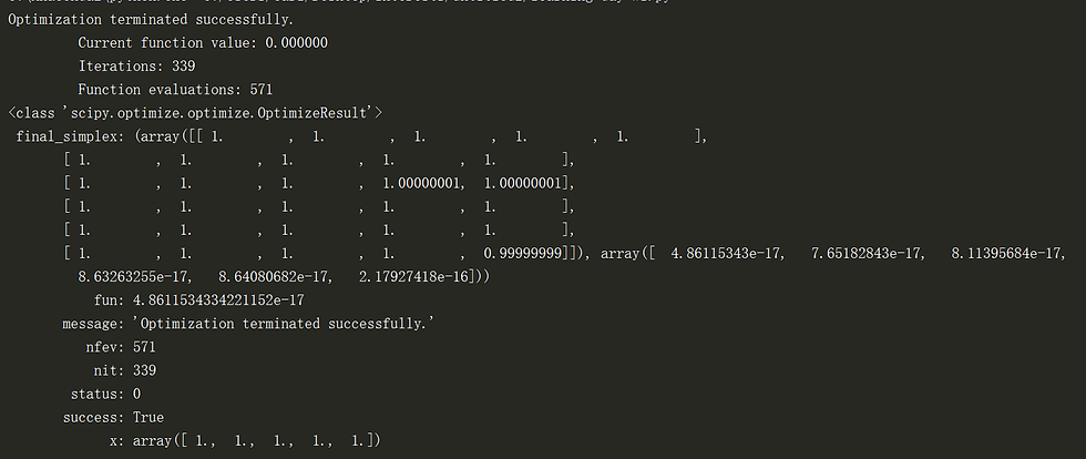
NM is an easy method to compute optimization problems, but it converge very slow(as you can see in the summary: iteration times). However, it is still pretty cool when dealing with some nice function like Rosenbrock func.
Here is how I did it.
**************************************************************************
import numpy as np import math import scipy.stats as stats import scipy.optimize as opt
def rosenbrock(x): return sum(100*(x[1:]-x[:-1]**2.0)**2.0+(1-x[:-1]) **2.0 )
x_0=np.array([1.3,0.7,0.8,1.9,1.2]) result=opt.minimize(rosenbrock,x_0,method="nelder-mead",options={"xtol":1e-8,"disp":True}) print type(result) print result
****************************************************************************

#Broyden-Fletcher-Goldfarb-Shanno Algorithm
In numerical optimization, the Broyden–Fletcher–Goldfarb–Shanno (BFGS) algorithm is an iterative method for solving unconstrained nonlinear optimization problems.
The BFGS method approximates Newton's method, a class of hill-climbing optimization techniques that seeks a stationary point of a (preferably twice continuously differentiable) function. For such problems, a necessary condition for optimality is that the gradient be zero. Newton's method and the BFGS methods are not guaranteed to converge unless the function has a quadratic Taylor expansion near an optimum. These methods use both the first and second derivatives of the function. However, BFGS has proven to have good performance even for non-smooth optimizations.
(Wikipedia)
The BFGS method requires gradient of the function, so before utilize that method we have to first calculate the gradiend. Again, us Rosenbrock for example:

It's gradient is :

then we use the gradient information along with the function information in the optimization function. And we can see in the output picture below, it only takes 52 times iteration to compute the optimization result, much faster than NM method which takes more than 300 iterations!
******************************************************************************************
import numpy as np import math import scipy.stats as stats import scipy.optimize as opt x_0 = np.array([0.5, 1.6, 1.1, 0.8, 1.2]) def rosenbrock(x): return sum(100*(x[1:]-x[:-1]**2.0)**2.0+(1-x[:-1]) **2.0 ) def der_rosen(x): xm=x[1:-1] xl=x[:-2] xr=x[2:] der=np.zeros_like(x) der[1:-1]=200*(xm-xl**2)-400*(xr-xm**2)*xm-2*(1-xm) der[0]=-400*x[0]*(x[1]-x[0]**2)-2*(1-x[0]) der[-1]=200*(x[-1]-x[-2]**2) return der
result=opt.minimize(rosenbrock,x_0,method="BFGS",jac=der_rosen,options={"disp":True} ) print result
*************************************************************

#3 Newton-Conjugate-Gradient algorithm
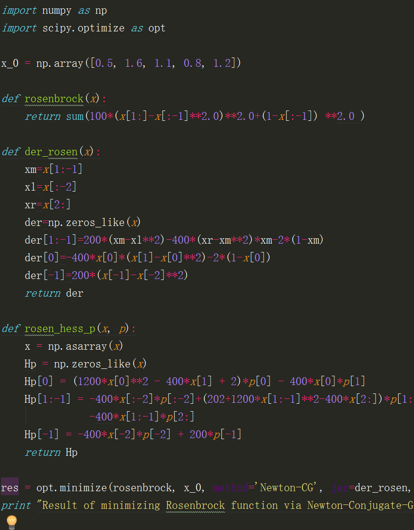
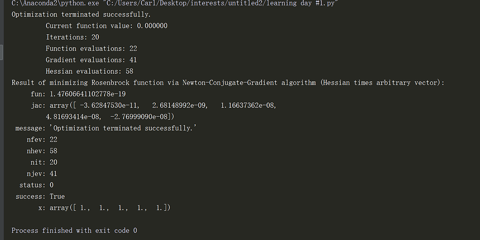
This method is even faster than the previous one. But to use this method, we have to calculate the Hessian matrix (, which is the second-order derivative matrix).
Its idea could be understood in this way:
First, using Tylor Expansion upon the function (2rd order):

where H(x0) is our Hessian matrix, and if it is a positive definite matrix we can have:

We can compute H matrix in this way:

where the boundary conditions are specified by:

*************************************************************************
import numpy as np import scipy.optimize as opt
x_0 = np.array([0.5, 1.6, 1.1, 0.8, 1.2])
def rosenbrock(x): return sum(100*(x[1:]-x[:-1]**2.0)**2.0+(1-x[:-1]) **2.0 )
def der_rosen(x): xm=x[1:-1] xl=x[:-2] xr=x[2:] der=np.zeros_like(x) der[1:-1]=200*(xm-xl**2)-400*(xr-xm**2)*xm-2*(1-xm) der[0]=-400*x[0]*(x[1]-x[0]**2)-2*(1-x[0]) der[-1]=200*(x[-1]-x[-2]**2) return der
def rosen_hess_p(x, p): x = np.asarray(x) Hp = np.zeros_like(x) Hp[0] = (1200*x[0]**2 - 400*x[1] + 2)*p[0] - 400*x[0]*p[1] Hp[1:-1] = -400*x[:-2]*p[:-2]+(202+1200*x[1:-1]**2-400*x[2:])*p[1:-1] \ -400*x[1:-1]*p[2:] Hp[-1] = -400*x[-2]*p[-2] + 200*p[-1] return Hp
res = opt.minimize(rosenbrock, x_0, method='Newton-CG', jac=der_rosen, hessp=rosen_hess_p, options={'xtol': 1e-8, 'disp': True}) print "Result of minimizing Rosenbrock function via Newton-Conjugate-Gradient algorithm (Hessian times arbitrary vector):"
print res
************************************************************************************

I will be posting optimization with constrains in next post!!!!


留言