Monte Carlo Pricing Method of European Call (Python)

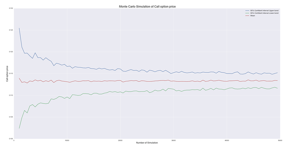
Assuming the underlying stock follows the geometric Brownian process, with some easy Ito calculus, we can actually produce perfect Monte Carlo estimator of the E call option. I omitted the calculus part, since it is trivial. Below is the code and the estimator convergence speed result:

*******************************************************************

#encoding=utf-8 import numpy as np import time from scipy.stats import norm import matplotlib.pyplot as plt import seaborn as sns from math import*

def GORB(a): if a<5: return "soso" else: return "too slow!"

#B-S parameters : S=2.45 K=2.50 t=0.25 r=0.05 sigma=0.25 # Portfolio=range(0,5000,500)

def BS(S,K,t,r,sigma): d1=(log(S/K)+(r+0.5*sqrt(sigma))*t)/(sigma*sqrt(t)) d2=d1-sigma*sqrt(t) return S*norm.cdf(d1)-K*exp(-r*t)*norm.cdf(d2)

def npBS(S,K,t,r,sigma): d1=(np.log(S/K)+(r+0.5*sqrt(sigma))*t)/(sigma*sqrt(t)) d2=d1-sigma*sqrt(t) return S*norm.cdf(d1)-K*exp(-r*t)*norm.cdf(d2)

def func1(S,t,r,sigma): plt.figure(1) sns.set_style("ticks") time_series=[] for i in Portfolio: strike_series=np.linspace(2.0,3.0,i) time_now=time.time() for x in range(i): BS(S,strike_series[x],t,r,sigma)

time_series.append(time.time()-time_now)

plt.bar(Portfolio,time_series, color="red",width=200) plt.plot() plt.show() plt.title("Computation running time of option's portfolio-Loop method") time_series=np.asarray(time_series) print "for loop运行时间（s）:",time_series.sum(),"。。。血崩" def func2(S,t,r,sigma): time_series=[]

for i in Portfolio: strike_series=np.linspace(2.0,3.0,i) time_now=time.time() npBS(S,strike_series,t,r,sigma) time_series.append(time.time()-time_now)

plt.bar(Portfolio,time_series, color="red",width=200) plt.plot() plt.title("Computation running time of option's portfolio-Numpy method") plt.show()

time_series=np.asarray(time_series) print "vector运行时间（s）:",time_series.sum(),"。。。有点吊"

# func1(S,t,r,sigma) # func2(S,t,r,sigma)

# Stock price follows geometric brownian motion, pricing call option using monte carlo def MonteCarlo(S,t,r,sigma,K,path): raw_simulators=norm.rvs(size=path,loc=(r-0.5*sigma**2)*t,scale=sigma*sqrt(t)) raw_simulators=S*np.exp(raw_simulators) simulators=np.maximum(raw_simulators-K,0.0).sum() price=exp(-r*t)*simulators/path return price

# print MonteCarlo(S,t,r,sigma,K,10000)

def MonteCarloConvergenceSpeed(S,t,r,sigma,K): size=100 pathscenario=range(1000,50000,500) UpperBond=[] LowerBond=[] mean=[] timemark=time.time() for path in pathscenario: result=[] for simu in range(size): result.append(MonteCarlo(S,t,r,sigma,K,path)) result=np.asarray(result) mean.append(result.mean()) LowerBond.append(result.mean()-1.96*result.std()) UpperBond.append(result.mean()+1.96*result.std()) line_table=np.asarray([UpperBond,LowerBond,mean]).T plt.plot(pathscenario,line_table) plt.title(" Monte Carlo Simulation of Call option price",fontsize=20) plt.xlabel("Number of Simulation",fontsize=15) plt.ylabel("Call option price",fontsize=15) plt.legend(["95% Confident interval Upper bond","95% Confident interval Lower bond","Mean"],fontsize=12) timemark=time.time()-timemark